


While studying behavior of dynamical systems phenomenologically - that is not by delving into their internal machinery, but instead considering only abstract collections of their properties, changing over time - we, following fundamental principles of mathematical modeling, tend to explain causes of changes of states of the properties by existence of certain dependence relations of the states of properties on changes of states of the same or some other properties; and, optionally, on the effects of external systems or the environment.
The objective of this page is to introduce Qualitative Dynamical Systems Mathematical Modeling Technique, developed as part of the Kaleidoscope Project, and to describe modeling solutions proposed by the Technique. The purpose of this technique and its solutions is to enable the creation of qualitative systems simulation models, capable of reproducing the behavior of existing or being designed qualitative dynamical systems.
Reproducing Behavior of Qualitative Systems
With the Help of Their Models
Reproducing, or, in other words, simulation modeling of behavior of dynamical systems, is a process of recreating, in a model, changes of states of properties of the modeled system, happening over time. Therefore, the organization of the process of reproducing behavior of these systems presumes creating models capable of generating sequences of changes of state of variables of the models similar to the sequences of changes of state of properties observed in the modeled systems.
So, since, by definition of the dynamical systems, all the changes in their state are explained by the changes in the state of the systems happened earlier, the process of reproducing behavior of a particular qualitative dynamical system carried out with the help of its simulation model should be performed as the sequence of transformations of current state of the model into its next state. In practice, this process, thus, should begin with the transformation of the initial state of the model, performed at the initial moment of simulation t = 0, into its state observed at the next moment in time, which can be denoted as t = 1. Then the state at time t = 1 should be transformed into the next state observed at the next moment t = 2. And then the process should continue as a systematic repetition of steps of transformations at the moments t = 2, 3, 4, 5, etc., as long as this makes practical sense.
Suggested description creates an understanding of the role of models in the technique of simulation modeling of behavior of qualitative systems. But it says nothing about how the models of this kind should be defined and how they should perform transformations of the current states of the models into their next states. Meanwhile, qualitative dynamical systems are the instances of the class of dynamical systems whose changes of states are determined by the dependence relations of states of properties of the systems on the combinations of states of groups of properties characterizing situations. Therefore, it is assumed that:
(1) following the general technique of modeling dynamical systems any particular model of a qualitative system should be defined as a collection of n variables xi, where index i of variable x runs from 0 to n-1; variables should represent qualitative properties of the modeled system; and values of the variables should be taken from a mathematical set, characteristics of elements of which make it possible to use them for representing states of qualitative properties; and that respectively:
(2) mechanism of computation of the states of the variables of the model has to be defined as the system of n equations, written as: xit+1 = f(argst), where: xit+1 is the state of the variable xi at the time t+1; argst stands for the list of arguments of the function f, holding values of groups of variables of the model at time t; and f is the function computing value of variable xit+1, as the dependent element of the dependence relation corresponding to values of independent variables of the relation, passed to the function as its arguments.
Presented on this page, the modeling technique has been developed as a complex of modeling solutions enabling the creation of qualitative system models in the form of a system of algebraic equations. Those solutions are based on the general principles of mathematical modeling of dynamical systems, mentioned above, on the one hand, but also reflect the discrete nature of qualitative properties and the character of behavior of qualitative systems, described on the page "Qualitative Dynamical Systems, Their Behavior, and Mathematical Modeling", on the other hand.
The following sections describe all modeling solutions, constituting the Modeling Technique, as well as examples illustrating the application of the solutions for writing state equations of the variables in the form of algebraic equations.
Domain Set of Mathematical Models of
Qualitative Systems
Creation of mathematical models of dynamical systems in the form of collections of variables assumes having mathematical sets, the nature of elements of which makes it possible to use them as the values of variables, denoting states of properties of the modeled systems. Thus, for example, the technique of creating models of quantitative systems utilizes sets of integer, real, or complex numbers, elements of which are used to denote the magnitude of modeled properties. On the other hand, techniques of modeling either logical or discrete systems, propositions of which may take only two states, use sets consisting of only two elements, such as "yes" and "no", or "1" and "0", depending on the adopted interpretation.
In contrast, the qualitative systems are neither quantitative nor logical. By assigning to properties of these systems different qualitative assessments of their states, we assume that properties are multivalued and may take different qualitative states at different times. And, thus, the elements of the set which should be used as values of variables, representing qualitative states of properties, will serve as unique markers of different qualities of the properties. Respectively, the markers are not supposed to have any associated connotations and interpretations. And, hence, the only relation that can be defined on such a set should be the equivalence relation of each element of the set to itself, and its non-equivalence relation with all other elements of the set.
Such a set can certainly be a set of signs. These signs can be either the letters of the alphabet of a language, used for description of the model in the form of text, or the codes of different colors, used when the model and the states of its variables are depicted graphically.
So, the definition of the set of signs used on this page is the following:
The Mathematical Set of the models of qualitative systems is the collection of uninterpreted uppercase letters of the Latin alphabet, and, thus, is defined as: D = {A, B, C, ..., Z}. Being a collection of elements which are used for representing values of arguments of functions and values of variables computed by the functions, set D serves in the models as the domain and the range of the state functions of variables of the models.
Remark 1. The definition of a set of models in the form of the set of colors, which in the context of creating qualitative systems, graphical models are called a Palette, is given on the page "Multicolored Logical Net Modeling Formalism".
Remark 2. Technique of description of process of computation of next state of variables of the models in the form of mathematical expressions written as a composition of algebraic operations, that requires having a carrier set allowing definition on it operations necessary for computing algebraic expressions, is described later in the sections of this page, devoted defining content of the state functions of variables of the models.
Qualitative Model Behavior Specification
Whatever the modeled qualitative system may be - whether existing in reality, or (when it is designed) present only in our imagination, creating its model assumes having a detailed specification of the dependence of states of each variable of the model on the states of various groups of variables characterizing situations that can arise in the model. And since such models are created for reproducing the behavior of the modeled systems, the structure and the content of the specification of the model have to be based on observed, or assumed, dependence of states of each property of the system on the occurrence of situations in the system. This dependence is described on the previous page, "Qualitative Dynamical Systems, Their Behavior and Mathematical Modeling", in the section: Qualitative System Behavior Specification.
The Qualitative Model Behavior Specification (QMBSpec) follows the structure of the QSBSpec, in the sense that it is also defined as a list of the sub-specifications. However, in this case, those sub-specifications are not specs of dependence of individual properties, but the ones of dependence of individual variables. Meanwhile, unlike the QSBSpec (each element of which describes a single Correspondence of the proposed state of property to the expected situation), each element of the QMBSpec is defined as the pair: [name of the variable/list of all Correspondences]. In this structure, the Correspondences determine the dependence of all states of the variable of the pair on all expected situations.
Thus, in order to describe the content of the QMBSpec, elements of its list are named: State Variable Dependence Specification (SVDSpec). Variables in each SVDSpecs are named xi, and values of the variables are denoted by constants taken from the set D. The general form of the structure of the QMBSpec is presented in Figure 1.
Figure 1. Structure of Qualitative Model Behavior Specification.
In this Figure:
(1) QMBSpec is defined as the iterator through the list L ni=0 of n SVDSpeci.
(2) Each i-th SVDSpeci { xi : C cn(i)j=0 { } } is a pair, where the first element of the pair, xi, is the dependent variable of the SVDSpeci, whereas the second is the iterator through the list of Correspondences C cn(i)j=0, the number of which cn(i) depends on index i.
(3) Each i,j-th Correspondence { cvt+1i,j : S sn(i,j)k=0 { } is also a pair. In that pair, the first element cvt+1i,j belongs to domain set D. It is a constant value which is supposed to be assigned to variable xi as its proposed value, in response of the model to emergence of the i,j-th situation S sn(i,j)k=0, described in the second part of the pair.
(4) Each i,j-th situation S sn(i,j)k=0 is also a list, and each i,j,k-th element of the list is the pair described as { xi,j,k : evti,j,k }. The first element of the pair is the variable xi,j,k, and the second is the constant evti,j,k, which belongs to the domain set D. Thus, both the variable and the constant are the k-th elements of the i,j-th situation of the i,j-th Correspondence of the i-th variable of the specification QMBSpec.
To summarize. Conversion of the QSBSpec to the QMBSpec is accomplished by replacing unique identifiers used in the QSBSpec with the names of the variables suggested by the modeling technique, and the identifiers of states of the properties with the elements of the domain set D, chosen to represent states of properties.
State Functions of Variables of Models of Qualitative Systems
To define a function, in a general sense, means to suggest a way for computing its values for all possible combinations of values of its arguments. Respectively, in order to define state function of a variable of a model of qualitative system (intended for reproducing changes of state of the modeled property observed in a modeled system), it is necessary to define a computation procedure of the function, capable of producing values of the variable for all possible combinations of values of groups of variables of the model, characterizing situations which are described in the Correspondences of the SVDSpec of the variable being computed and which ought to be passed to the function as its arguments.
However, in order to construct such a computation procedure, it is necessary to take into account that the suggested way for its computing must ensure obtaining results despite the challenges caused by the characteristics of dependence of states of variables of models of the qualitative systems on irregularities of the occurrence of situations in those systems.
Content of Computation Procedure of State Functions
of Variables
Being, by their nature, the systems of simultaneously acting components which produce asynchronous and fragmentary changes in the state of properties of the systems, both the qualitative systems and their behavior are characterized by the fact that, the all transformations of state of properties of the system into their next state, performed at any particular moment in time, are really caused by not all, but only the part of all the variety of situations that can emerge and be present in a system.
This statement actually means that since concrete content of situations can be formed in the model only immediately before computing each of its functions, and thus that the knowledge on which of the situations, expected by the function, must be passed to it as arguments and which are not, cannot be obtained until its computation begins, absolutely all groups of variables listed in the SVDSpec, must be included in the list of arguments of state function of each variable; so to say just in case. And, thus, because of that, it turns out that, not all, but only those groups of arguments that at the moment of computation of the functions, characterize expected situations, can be used for computing values of functions (and their variables) corresponding to the expected situations.
Hence, taking into account all that has been said by now, in order to compute the function, its procedure (that can be also referred as the algorithm) have to be enabled for: a) systematic scanning all groups of arguments of the function for identifying among them expected situations; b) producing either the real proposed values of the variable taken from the Correspondences of the Specification in cases when a single, or a few, expected situations are detected in the arguments, or, alternatively, producing proposed values marked with some auxiliary symbol that should be used to denote produced proposed value as undefined; c) generating final proposed value of the function out of all proposed values (defined or undefined), assuming that it may come out as undefined in cases when either none of the expected situations are present in the model, or when two or more existing situations produce different proposed values and, thus, create uncertainty in choosing a single value of the function; and, at the end, d) sorting out cases when final proposed value turned out undefined and leaving computed variable unchanged, when it does.
Proposal for Implementation of State Functions of
Variables in the Form of Algebraic Expressions
If a model of a qualitative system were created as a computer program, then each of its functions, based on the understanding of its content, described above, would most likely be implemented in the form of a loop through all groups of its arguments, characterizing different situations expected by the function. Whereas, each iteration of the loop could begin with the test if the situation, being processed, is present in the state of the model, and perform computation of the value of the function by checking the state of data and executing computational operations depending on whether the situation is present or not.
However, when creating mathematical models of qualitative systems, whose functions should be defined as algebraic expressions, we have to deal with such a kind of computation, dataflow, which, so to speak, is laminar. And, thus, it can develop only in one direction - from the values of independent elements of the dependence relation of the variable, i.e., from the arguments of the function (leaves of the computation tree) to the dependent element of the relation, i.e., the computed value of the function (root of the computation tree). It is obvious that this process cannot contain any cycles, and branching out in order to execute some computational operations while bypassing others, depending on the state of the data.
Described in this section approach to computing a function in the form of an algebraic expression is an experimental attempt to fit into an inherently linear process of sequential execution of operations of algebraic expression, all such features of algorithms as: cycles, dynamic computation of estimates of states of data, and conditional choices for executing some operations while bypassing others; which usually make structure of algorithm quite branchy.
From Computer Algorithm to Algebraic Sequential Computation
Unlike description of behavior of quantitative systems, nature of computing next state of which lies in the transformation of quantitative values of arguments of functions into the quantitative value of the function, i.e., literally in physical modification of quantities, characterizing states of properties of quantitative systems, the essence of computing transitions of qualitative systems from state to state, is the replacement of some qualitative estimates of state of properties with other qualitative estimates. And this difference, in the content of the process of these computations, opens up a fundamentally new way of describing the computational process of the functions of the qualitative systems.
All observed changes of variables of models of qualitative systems are generally explained by the discrete nature of these systems, fragmentary changes of state of their properties, and asynchronous occurrence of the situation in the systems (and their models). However, these factors can create challenges when calculating the algebraic expressions of the functions. They arise because not all but only some of the situations described in the specifications of the state equations of the variables actually exist in the model (and in the groups of arguments of the functions) at the moment of computing the functions, and also because of what particular proposed values the expression computes as a response to the appearance or disappearance of situations in the model. And these challenges must be resolved.
But the mathematical model of a dynamic system is just a collection of state equations of the system, and nothing more. Therefore, this proposes that the resolution of challenges should occur not outside but inside the algebraic expression, and be provided by the operations used for computing the expression. Thus, as it was shown by the study, the feasibility of implementing functions of models of qualitative systems in the form of algebraic expressions is determined by the approach to constructing algebraic expressions of functions, that makes the challenges surmountable. This approach and its solutions are described below.
(1) Since in accordance with the specification, any single states of a variable may
depend on existence of several different situations and all the variety of situations
that may cause change of all states of the variable can, in the worst case, emerge
independently, it is possible that during each computation of the function either
none or only a part of all expected situations may be present in the groups of the
arguments of a function. Therefore.
(2) Dependence of a value of a function on several situations assumes that the
process, computing values of a state variable of a model, should a) contain
operations which produce proposed values corresponding to situations described
in the specification of the state variable, and b) an operation that analyzes
the obtained proposed values and selects from them the only final value of the
function. Therefore.
(3) Since the state of the model is constantly changing from iteration to iteration
and, thus, any knowledge about changes of situations is represented in the model
only by the state of its variables, revealing which of the situations, expected by
the expression, are present and which are absent, at the time of its computation,
can only be carried out by the expression itself. Therefore.
(4) Since the estimates of the data state, originally created to control the course
of the computation process, may later be used instead of defined values that were
for some reason not computed, i.e., as the markers of undefined values, the values
used as the markers of the estimates should be taken from another set, elements of
which should be considered as auxiliary and be compatible in type with the elements
(i.e., symbols) of the set D. Therefore.
(5) The technique of computing algebraic expressions does not assume the presence of any
variables in the expression. Dataflow, in them, is distributed from the output of
any executed operations directly to the input of the following operation, and so on.
However, the operations used for computing XDNF expressions can yield results whose
values are taken either from the set D or the set X, and take
elements of both types as their operands as well. Therefore.
Meaning of the Elements of Set X
(o) The symbol "!" must be used to denote the fact of presence of the expected situation in the group of arguments of the expression;
(o) the symbol "$" must be used to denote the fact of absence of the expected situation in the group of arguments of the expression, and also either as a proposed value when this value is indefinite because the situation that could produce it turned out to be absent, or as a final proposed value when it is indefinite because simultaneously all situations expected in the expression turned out to be absent and as a result none of the proposed values of the variable was computed;
(o) and the symbol "#" shall be used to denote a final proposed value when it cannot be determined because, in the process of computing that value, it was discovered that two or more proposed values were different and thus a conflict of variable values arose, which prevented the final value from being computed as determined.
Examples of the interpretation of the meaning of elements of the set X can be expressed in the form of different statements. Instances of the qualitative assessments of state of a computational process are: "Situation recognized", "Situation not recognized", "Proposed value not defined", "The final value of the function is not defined as none of the expected situations is present in the state of the model", or "The final value of the function is not defined as a contradiction of proposed values is detected".
Described above assumptions of possibility defining functions in the form of the XDNF expression and utilizing, in addition to the earlier defined domain set D, an auxiliary set of symbols X turned out to be not just useful, but the major key factor terning the described trial approach into a real modeling solution of the qualitative systems mathematical modeling technique.
Homogeneous Carrier Set of Model and Family of
Hybrid, Binary Operations Closed on the Set
As it was shown by the study of feasibility of defining functions of models of qualitative systems in the form of the algebraic expressions, homogeneity of the sets D and X, arising in the result of defining both of them as sets, whose elements are symbols, creates a unique opportunity to define the carrier set of the functions of a model as the union of these two sets.
So, the definition of the carrier set of the model as the homogeneous, i.e., as S = D U X, based on the definition made, in turn, makes it possible defining on the set S a family of hybrid, binary, and closed on the entire set, operations, whose operands are capable of taking either the elements of the set D or the elements of the set X and producing any element of the set S.
Research on the feasibility of defining, on the set S, operations capable of performing the required computation was conducted. And its result made it possible to construct five hybrid operations, allowing the implementation of the procedure of computation of state functions of variables of qualitative systems models in the form of an extended disjunctive normal form of the algebraic expression written as a composition of these operations. The names, denoting symbols, and comments on the roles of the operations in the process of computation of the expression are listed in Table 1.
| Name | Sign | Meaning |
|---|---|---|
| Equivalence | ? | Compares operands; yields "!" when operands are equal, or "$" when they are not. |
| Conjunction | & | Works as a boolean AND operation for symbols "!" and "$". It is used to compute n-ary Conjunction. |
| Production | * | Produces proposed values for all identified or not identified expected situations. |
| Disjunction | | | Analyses all proposed values, chooses final value. It is used to compute n-ary Disjunction. |
| Application | < | Checks if the final value is an element of set D, and returns it; otherwise returns the current value of the variable. |
The table lists all five operations in the order they are used in the expression. Names of the operations are presented in the first column of the table. The second column contains symbols used to denote the operations in an expression, where the operations are written in their infix form. And the third column provides a brief description of the operations.
Complete description of the sets D, X, and S, as well as of the five operations defined on the set S, that all together constitute the algebraic system, is presented on the page "The Algebra of Symbols".
General Form of a State Equation of a Model Defined
as the Expanded Disjunctive Normal Form - XDNF
The general form of a state equation of a variable whose right-hand side function is implemented as the XDNF expression written as a composition of hybrid operations defined on the model's carrier set S can be presented as a formula.

The arguments of this expression are variables representing the current state of a model and constants taken from the model variable dependency specification. They are passed to the function as: 1) a list gv, elements of which are groups of variable some concrete combinations of values of which can characterize situations expected by the function, 2) a list ev elements of which are groups of expected values of variables, given in the groups of array gv; they are used to recognize combinations of values characterizing expected situations that may be present in the groups of variable of array gv, 3) a list pv holding proposed values of computed variable, corresponding to the expected situations, and 4) a constant sv that serves as the spare value holding current state of the computed state variable, which should be used when computed value turns out be undefined.
Computation of Expanded Disjunctive Normal Form Equation
Computation of this equation can be described as performing the Disjunction operation that yields the value of the function obtained as a result of processing all proposed values generated as a result of computing all terms of the expression. Whereas the computation of each particular term is accomplished as execution of the Production operation that generates proposed values of the variable either as a constant taken from the array pv, when the expected situation is recognized, or as the auxiliary symbol $, when the situation is not recognized. Meanwhile, the recognition is carried out by two operations: Equivalence and Conjunction. First of them - Equivalence performs by-element comparison of the variables of the group of array gv with their expected values represented by the constants in the groups of array ev. And the Conjunction operation is used to confirm that all results of the comparison of all elements of both groups of both arrays are compared, and, thus, the situation can be deemed recognized.
Ultimately, since (as it was discussed earlier) the final proposed value yielded by the Disjunction operation may be undefined, the last operation that completes the computation is the Application operation; it is denoted by the symbol "<". This operation checks the result of the Disjunction operation and, in the case when it is undefined, uses the value of the last spare argument of the sv function, containing the current value of the computed variable, instead of the undefined result of computation. And, as a consequence of this replacement, the computed variable of the equation receives the same value that it already holds again and, thus, effectively remains unchanged.
XDNF Expressions Calculator is presented on the page "Extended Disjunctive Normal Form Expression Calculator".
A more detailed description of the process of computation of the XDNF expression is provided in the two following sections. They present several examples of computing the only expression with different values passed to it as arguments. The examples are used for illustrating and describing steps of the execution of the expression, so to speak, in the "debugging" mode.
Illustrative Example of State Equation and
Process of Computation of
the State
Variable of the Equation
This section presents the process of creating a model of a qualitative dynamical system as a sequence of steps: creating a description of the behavior of a modeled system in the form of QMBSpec, and creating a model of a qualitative system based on QMBSpec. Then it demonstrates the process of using the created state function of the variable on the example of four experiments of computation of the value of the state variable of the model for different initial states of the variable and arguments of the function computing different states of the variable for different arguments.
Example of State Equation Implemented as the XDNF
Expression
A presented example of an equation defined by the above formula describing the dependence of values of a variable "x0" on the combinations of values of variables x1, x2, and x3, which characterize two situations (x1) and (x2, x3) that may arise in a particular system, is presented as an equation.
x0 = x0 < [ ( P * (x1 ? E) ) | ( H * ( (x2 ? M) & (x3 ? Q) ) ) ]; (1)
This simple equation states that the two values that variable x0 can take are determined by two situations and hence two correspondences. The first, from left to right, Correspondence describes that variable x0 should take value P when the value of variable x1 is E, whereas the second Correspondence describes that variable x0 should take value H when the value of variable x2 is M, while the value of variable x3 is simultaneously marked by symbol Q. Despite such simple dependence, different combinations of values of independent variables (arguments) of the expression: x1, x2, and x3 may cause the expression to be computed with different results and thus would create at least three different values of the variable x0. All these cases are considered and illustrated in the next section, which describes every single step of the computation of the expression in all the details.
Computation of the State Variable of the XDNF
Equation
The content of the illustrations, presented in this section, is based on the simple equation (1), the right part of which is defined as the XDNF expression. Four different ways of computing this equation are illustrated as four examples: A, B, C, and D.
All four examples illustrate the process of computing the value of the dependent variable x0 of the equation, with four different combinations of values of two groups of arguments, where the first group consists of variable x1, while the second one consists of variables x2 and x3. Each of the examples is shown as seven lines. Therefore, to show how the expression computes different results, the first line presents the result of initialization of the computed value x0 with the same value G in all examples, but variables x1, x2, and x3 with different values in each example. The second line is the initial state of the equation. Lines three through six present results of the execution of operations: Equivalence, Conjunction, Production, and Disjunction. And finally, the seventh, and the last, line presents the result of the execution of the Application operation, which is the final proposed value of the variable x0 computed by the expression.
Below is the first example, A, followed by the detailed description of the steps of executing these operations.
Detailed Description of the Roles of the Operations
and Steps of Computation of Example A
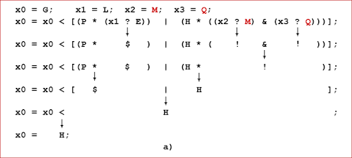
Figure 2. Example A. The application of these operations is depicted in this figure by arrows drawn from the signs of operations to their result.
This figure provides a detailed description of the steps of the computation of the expression. It illustrates a case when the arguments of the expression are initialized as: x0 = G; x1 = L; x2 = M; x3 = Q. Accordingly, the situation (x1) is not present and not recognized, whereas the situation (x2, x3) is present and recognized. Therefore, the only proposed value "H" produced by the Production operation, as the correspondence to the situation (x2, x3), is the one that can be chosen by the Disjunction operation as the final proposed value and then accepted by the Application operation. So, that value "H" becomes the value of the variable x0.
Step 1. Equivalence operation is defined as yielding an auxiliary symbol "!" of set X when both of its operands are represented by the same symbol of set D, or another auxiliary symbol $ of set X when the values of the operands are different. Therefore, in the context of this example, the Equivalence operation is used to compare value of argument x1 with its expected value, and yields symbol "$", since this value is not the same as expected value "E"; as well as for comparing the values of the argument x2 and x3 with their expected value, and yields, in both cases, symbol "!", since both these values are the same as their expected values "M" and ?N?.
Step 2. Although the Conjunction operation is defined on a set whose cardinality can be much greater than 2, its application to operands and results that can only be the symbols "!" and "$" completely replicates the behavior of the well-known Conjunction operation defined on a set consisting of only two elements. Therefore, in the context of this example, the Conjunction operation is used only once. It takes the results of the Equivalence operation, each of which in this case is represented by the symbol "!", and produces the symbol "!", confirming that the expected situation is present in the model and, thus, is recognized.
Step 3. The task of the Production operation either consists in producing the proposed value of the variable corresponding to the recognized situation or in marking the produced proposed value with an auxiliary symbol indicating that the proposed value is undefined, when the situation is not recognized. Therefore, in the context of this example, Production operation takes its operands as the constant "P" and the result of recognition of the situation of the term, and yields symbol $ since the result of recognition of the situation is marked with symbol $, indicating that the situation is not recognized.
Step 4. This step is performed by the Disjunction operation, task which consists in choosing final proposed value of the expression that is determined by analyzing all proposed values produced by Production operation, taking into account that some proposed values may be defined while the otters undefined due to the absence of some situations; as well as marked as undefined by the operation itself. Therefore, in the context of this example, the Disjunction operation is applied only once. It takes two proposed values denoted by the symbols $ and H, and chooses from them the symbol H which outputs as the final proposed value of the expression.
Step 5. The role of the Application operation is obvious and is to yield either the computed value of an expression when it is defined, or the current value of the variable when the computed value is undefined. Therefore, in the context of this example, Application operation takes the final proposed value, computed by the Disjunction operation, as its one operand; the current value of the variable, as its second operand; determines that the final proposed value is represented by the symbol "N" and, thus, i s defined; and yields "N" symbol as the computed value of the variable, leaving the current value of the variable "G" unused.
Description of Computation of Examples: B, C, and D
The computation of the rest of the examples: "B", "C", and "D" follows the same schema of computation as was described for the first example "a", and are different only in the way of initialization of the variables: x1, x2, x3, that make the expression, despite the same operations and the same number of steps to compute the different values of the target variable x0 of the expression. That difference is explained by different internal analyses, conducted by the operations that make them produce different values of the variable corresponding to different situations present in the arguments of the expression, as they are initialized differently. These differences in the computation of expression are described for each example individually.
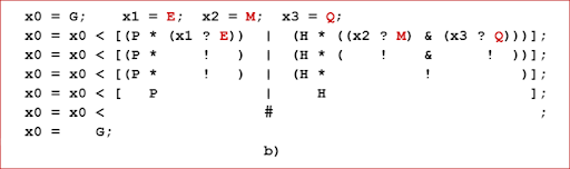
Figure 3. Example B.
This figure illustrates case when arguments of the expression initialized as: x0 = G; x1 = E; x2 = M; x3 = Q; These settings make both: the situation (x1) and the situation (x2, x3) are recognized, and, as the consequence of that, the produced proposed values "P" and "H" create uncertainty in choosing the final proposed value of variable x0. Therefore, the Disjunction operation marks the final proposed values by the symbol "#", indicating, thus, that it is not determined. And, in the end, the Application operation leaves the current value "G" of the variable x0 unchanged.
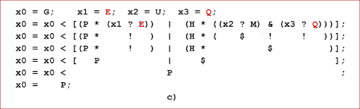
Figure 4. Example C.
This figure illustrates the case opposite to case A. Here, the arguments of the expression are initialized as x0 = G; x1 = E; x2 = U; x3 = Q; and this leads to the fact that the situation (x1) is recognized, but the situation (x2, x3) is not. Hence, the only proposed values "P", produced by the Production operation, can be chosen by the Disjunction operation as the final proposed value and become the value of the variable x0.
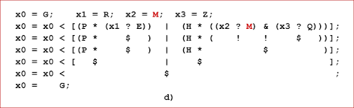
Figure 5. Example D.
This figure illustrates a case similar to case B. Here, the arguments are initialized as x0 = G; x1 = R; x2 = M; x3 = Z. This means that none of the expected situations are present in the arguments and, hence, none of them are recognized. So, both proposed values of the variable, produced by the Production operation, are represented by the auxiliary symbol "$". And therefore, similar to case B, the Application operation leaves the value of the variable x0 in its current state "G".