Here is What You Can Do on This Page

Select a predefined model to be simulated from the Model Chooser’s dropdown list. Use the three single-step buttons: "Micro Step", "Medium Step", and "Major Step", located in the upper row of the buttons, to execute equation simulation steps. Use the "Start/Stop Auto Simulation" toggle button to start or stop automatic repetition of simulation steps, either in the mode remaining after the last use of some single-step button, if any of them have been used previously, or in the "Major Step" mode, when none of the single-step buttons have been used yet. Use the "Reset Simulation" button to reset the simulation process to its initial state, letting it be executed again from the beginning.

Models That Can Be Chosen for Simulation

Prepared for the simulation, models may exhibit either self-driven or mixed self-driven and input-driven behavior. This behavior may also often be viewed as the process consisting of several independent sub-processes, which may demonstrate a chaotic, yet deterministic nature of behavior, observed in the systems. Identifying in such processes independent sub-processes may be quite difficult.

The purpose of this page is not to show how big a qualitative dynamical model can be, but to demonstrate the principle of transformation of the current state of the models into their next state. Therefore, all the models in this presentation are intentionally made of a limited size. These models are organized into three groups.

First group of models. Group "Full State Situations and Self-Driven Models" consists of two models. Each possible combination of all states of the state variables of the models of this group (presented as the State Vector of the equation) characterises a particular situation that may occur in the modeled systems.

Model-1.1 demonstrates a case when each state of the model is recognized as the situation to which the model responds by transitioning to the next state, corresponding to the situation.

Model-1.2 is a variation of Model-1.1 in which only some states of the model are recognized as situations to which the model should respond, but the others are not.

Second group. Group "Partial Situations and Input Driven Models" currently consists of only one model.

Model-2.1 demonstrates a case where all state variables of the model are split into two groups that may change independently. The model behavior, thus, is constituted of two independent processes. In order to present this clearly, one process is finite while the other is endless.

Third group. Group "Partial Situations and Mixed Input Driven Models" consists of one model:

Model-3.1 demonstrates a case where there are no explicitly separated processes. Instead, there is only one process in which unpredictably occurring partial situations are the causes of fragmentary, e.g., partial, changes in the full state of the model.

For Those Who Want to Know More

Observed behavior of a qualitative system is perceived as a process of occurrence of situations in the system and its reactions to these situations, expressed in the execution of actions that change the state of some properties of the system. Therefore, the task of the model, reproducing the behavior of a qualitative system, is to systematically recognize situations represented by combinations of states of groups of variables that have arisen as a result of the previous behavior of the model and to make changes in the current state of the model corresponding to the recognized situations.

The solution to modeling the behavior of qualitative systems, presented on this page, is given in the form of a vector state equation describing the process of computation of the correspondences "Situation -> Change of the State of Properties" as a composition of vector operations and matrix transformations of the current state of the model into its next state. The structure of the state equation and description of the process of its computation are described in the sections to follow.

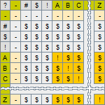
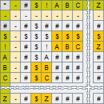
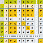
Parts of the Qualitative Dynamical System Equation

The equation consists of eight elements listed in the order of their invocation in the computation, i.e., from right to left.

1. External Input Vector has ___ background and is an optional element of the model. It is included in the model in the case when the modeling technique requires the model simulation process to be driven by external input, and is omitted otherwise.
2. Current State Vector has ___ background and is the representation of the state of the model at the moment t, i.e. at the time when the iteration of simulation is going to begin.
3. Recognition Matrix has ___ background and is the Current State Vector transformation operator. The number of columns in this matrix corresponds to the number of elements of the Current State Vector of the model, whereas the number of rows is determined by the number of situations that are supposed to be recognized and which, for that purpose, have to be described as the columns of the matrix.
4. Recognized Situations Vector has ___ background and is the result of transformation of the Current State Vector of the model. It holds symbols indicating facts of recognition of the presence of expected situations in the Current State Vector of the system.
5. Generation Matrix has ___ background and is another transformation operator. It is applied to the Recognized Situations Vector and generates values of the Proposed State Vector. Each column of this matrix, thus, is associated with the particular recognized situation, and each row with the particular element of the Proposed State Vector.
6. Proposed State Vector has ___ background and is the result of Generation transformation. It is a collection of changes that should be infused into the Current State Vector. At the moment of computation of iteration, some of the expected situations may exist while some others might not; the Proposed State Vector may be partially defined. Some of its elements may hold symbols denoting the valid state of the variables of the model, whereas others may appear to be just the auxiliary symbols used in the process of computation, indicating that the expected situation was not recognised and, therefore, the computed value is not defined.
7. Dobbed State Vector has ___ background and is a clone of the Current State Vector. It is presented here for just convenience to have one more view of the Current State Vector right in the place where it and the Proposed State Vector are used as the arguments of the vector operation computing the content of the Next State Vector of the model.
8. Next State Vector has ___ background and is the result of infusion of the Proposed State Vector with the Dobbed State Vector. This is a temporary vector that is needed to present the computed result of an iteration - values of the Current State Vector at the time t+i, where i is the number of the completed iteration. Values of the elements of this vector are copied to the corresponding elements of the Current State Vector as soon as a step button is clicked, and the simulation process proceeds to the initial state of the next iteration.

Representation of Values of the Elements of the Parts of the Equation

It is assumed that all values of state variables, which in the state-space representation of the model are defined in the form of the elements of the Current State Vector, are qualitative and therefore can be denoted by symbols taken from a certain set of symbols. On this page, this set of symbols is defined as the set of uppercase characters of the Latin alphabet.

There are two sets of symbols that are used to represent the state of the model under simulation: a set of domain symbols and a set of auxiliary symbols. The set of domain symbols D is defined as:

D = { A, B, C, …, Z, … },

and the set of auxiliary symbols X, defined as:

X = { -, !, $, # }.

Symbols of set D are used to denote values of elements of the model representing states of the properties of the modeled system. And the symbols of set X are used to denote values of those elements of the state of the model, which represent the state of the process of computation of the equation. The meaning of the symbols of the set X is the following:

Symbol “-” is a kind of “zero” of the algebra used for computing the models and is used to represent the values of those elements of the vectors and the matrices of the equation, which should be excluded from the process of computation.

Symbol “!” is used to denote one of two possible results of the procedure of recognition of a situation (see a description of application of the Equivalence and the Conjunction operations described below in the section: "Computation of Matrix Equation of Model of Qualitative Dynamical System"). It is yielded to present the fact asserting that a particular value presented in a particular element of the Current State Vector of the model has compared to its expected value presented in a particular element of a particular row of the Recognition matrix and thus the compared element of the Current State Vector is considered as the recognized element of the expected situation.

Symbol “$” is used to denote the second possible result of the recognition of a situation. It is an alternative to the symbol “!” and serves for presenting the fact of asserting that a particular value presented in a particular element of the Current State Vector of the model was not compared as the expected value presented in a particular element of a particular row of the Recognition matrix and thus the compared element of the Current State Vector cannot be considered as recognized.

Symbol “#” is to denote a particular result of the Generation transformation (see a description of application of the Production and the Disjunction operations described below in the section: "Computation of Matrix Equation of Model of Qualitative Dynamical System"). It is yielded by the Disjunction operation to eliminate the conflict that may occur when two or more situations are simultaneously recognized by the Recognition matrix and then transformed by the Generation matrix to different proposed values.

Initialization of the Vectors and the Matrices

In order for the equation to be computed, its elements should be initialized. This initialization is conducted automatically right after the model is picked up from the Model Chooser dropdown list.

Initialization of vectors. The Current State Vector is initialized with the model's initial state provided by the specification of the chosen model. All other vectors are populated with the symbol “-” indicating that their elements are empty, as not yet computed.

Initialization of matrices. Following the general mechanism of application of the matrix operators, carrying out transformation of their input vectors into the output ones, by means of multiplication of the input vector by each row of the matrix, initialization of both matrices is determined by their roles in the equation.

(1) Initialization of the Recognition Matrix. The task of this matrix is to transform the Current State Vector of the model into the Recognized Situations Vector. Therefore, this matrix is initialized in such a way that its every row is filled with one of the expected combinations of values (elements of set D), which the Current State Vector may have, The rows, thus, characterize situations facts of occurrence or absence of which should be computed as the values of the Recognized Situations Vector, and to which the model should respond by changing value of one or more of its variables.

(2) Initialization of the Generation Matrix. The task of this matrix is to transform the Recognized Situations Vector into the Proposed States Vector. Accordingly, each row of the matrix is filled with the symbols (elements of set D) denoting proposed values of the variable, associated with that row. All these symbols are placed at the intersections of the row with the columns that are associated with the elements of the Recognized Situations Vector, indicating those situations on the occurrence of which values of the Proposed States Vector depend.

All elements of both matrices that are not initialized with any valid values taken from the set D are filled with the symbol “-” of the set X, denoting that at the time of computation of the equation, these elements do not represent any meaningful value for the model, and should be ignored.

Detailed technique of application of the matrices to the process of computation of the model state equations is described in the section: Computation of Matrix Equation of Model of Qualitative Dynamical System, located below.

Highlighting Active Vector Background and
Changes in the Status of Their Elements

As the simulation process is a sequence of computational steps of execution of vector or matrix transformations, there is always a vector toward which the currently executed operation is targeted. This vector is considered an active one. To emphasize the active status of such a vector, the background of the currently active vector is highlighted in pink.

When carrying out a simulation process, the Simulation Engine presents changes in the state of the elements of the active vector after every executed operation. For this purpose, each changed state element of the vector is highlighted with the color corresponding to the color of the current, i.e., the usual or the active background of the vector.

Computation of the Matrix Equation of the Model of
Qualitative Dynamical System

The process of computation of the equation consists of performing a sequence of four vector and matrix operations that transform the content of the Current State Vector of the model into its next state. Respectively, these operations are executed as four successive steps, which are carried out from right to left. They are.

Input Application Step. The input application, an optional step of computation of the equation, is involved in the case when the state of some properties of the modeled system can be changed by external effects. It is implemented in the model as executing the "Application" (<) operation, which "injects" the values of the External Input Vector into the Current State Vector of the model. This operation is expressed in replacing the values of the elements of the Current State Vector with the values of non-empty elements of the External Input Vector. The result of this operation is the modified Current State Vector.

First Computation Step. The task of the first computation step is the transformation of the Current State Vector of the model into the Recognized Situations Vector. It is carried out as multiplication of the Current State Vector by the Recognition Matrix, and is implemented as computation of each element of the Recognized Situations Vector by applying two "AoS operations: the Equivalence and the Conjunction".

First, the Equivalence operation is used to systematically perform the pairwise comparison of the elements of the row of the Recognition Matrix (corresponding to the being computed element of the Recognized Situations Vector) with the elements of the Current State Vector. The results of these comparisons can be either the symbol "!", meaning that the operands of the Equivalence operation have been compared, or the symbol "$", meaning that they have not been compared.

Second operation - Conjunction is applied to all results of the Equivalence operation. Its result can be represented by “!” symbol, indicating that all results of the Equivalence operation are represented as “!” symbol and, thus, that the situation described in the Current State Vector has been recognized, or, alternatively, as the "$" symbol which means that at least one of the results of comparison of values of the Current State Vector with its expected value described in the row of the matrix has not been compared and, therefore, the situation is deemed unrecognized.

Second Computation Step. The task of the second computation step is the transformation of the Recognized Situations Vector into the Proposed State Vector. It is carried out as the multiplication of the Recognized Situations Vector by the Generation Matrix. The technique of this multiplication is implemented as computation of each element of the Proposed State Vector by applying two "AoS operations: the Production and the Disjunction".

First, the Production operation is used to systematically take pairs consisting of the element of the row of the Generation Matrix (corresponding to the being computed element of the Proposed State Vector) and the element of the Recognized Situations Vector. The result of processing each such pair depends on the values of the elements of the pair and may be computed as one of the symbols: “-” or “$”, or as the element of the row of the matrix if it is a symbol of set D.

Then, the Disjunction operation is applied to all the results of the Production operation with the intention to choose out of all of them the single final proposed value that might be used as the next state of the element of the Proposed Values Vector. So, to achieve that goal, the Disjunction operation starts with assigning to the final proposed value its initial value as the symbol “$”, ignores all results of the Production operation, represented by the symbols "-" or “$”, and identifies cases when two or more proposed values appear as different symbols of the set D. In accordance with the definition of the model, the occurrence of different proposed values is considered contradictory, and to prevent this contradiction, the Disjunction operation marks the final proposed value with the symbol “#”.

Thus, in the result, it may always happen that the final proposed value holds either: a) the “$” symbol, when none of the expected situations are present in the state of the model and recognized; b) the "#" symbol, when the conflict of the proposed values is detected; and c) a symbol belonging to set D, when one, two or even more situations are recognized and all produced the same valid proposed value, which can be used as the value of the element of the Proposed Values Vector. Processing all three cases is accomplished by the last third step.

Third Computation Step. This computation step is the last in the process of computing the equation. It is accomplished by the Application operation. Its task is to check if the final proposed value is undefined and replace it with the value of the corresponding element of the Current State Vector.